The On Ramp/Level 1/Solve

Exporting to PHASTA

After the partitioning performed via Chef in the last steps, we now have the problem domain in a form that the PHASTA executable can read. In your 8-1-Chef directory, create a sub-directory named "Run". This will contain all of the simulation data from this case, which we will use in our PHASTA run. Remember that for this on-Ramp tutorial we have partitioned our case of interest to 8 parts. Therefore, we need to create a sub-directory named "8-procs_case" within the /8-1-Chef/Run/ directory. Once you have mkdir'd and cd'd into this new Run/8-procs_case/ subdirectory, make softlinks ("ln -s <path/file*>") to the N=8 restart and geombc "checkpoint" files that where constructed by Chef located in the 8-1-Chef/8-procs_case/ directory. When in the Run/8-procs_case sub-directory, a good command to do this is the following:

ln -s ../../8-procs_case/restart* .
ln -s ../../8-procs_case/geombc* .

Also create a numstart.dat file. This file will specify the time and timestep that the simulation has completed thus far. For our case, we have not yet run the simulation, thus our time and timesteps are 0 0. Use the following command in the "Run/8-procs_case" directory to create the numstart.dat file:

echo 0 0 > numstart.dat

Build the executable/specify runtime parameters

What remains is to determine the version of PHASTA to build and run. Since there are a bunch of researchers working on PHASTA at any given time, there are many branches/versions of the main code.

Note: You may not have access to the phasta-next repo yet. If that is the case, you can just use the regular phasta repo (by replacing all the "phasta-next" with "phasta" in these instructions).

Retrieve/build a version of PHASTA code

To have your first run of PHASTA, you will need an executable of the PHASTA code. There are many ways to do this, and below is intended to get you a generic executable. The many nuances to this proccess can be found on the Level 2 page here. Navigate to your home directory. Create and enter a directory here named "git-phasta". In a web browser, navigate to the online git repository for phasta-next and select the "clone" or "code" icon. The result should be similar to the following picture, where a pop-up gives a web address:

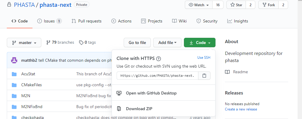
Copy this address and within the "git-phasta" directory execute the following command and enter your github credentials:

git clone https://github.com/PHASTA/phasta-next.git

After this is finished there will be a subdirectory created named "phasta-next" that contains the code tree that you wish to build. Back within the git-phasta directory create another subdirectory named "build_phasta-next". Now we must set the environment so that the compiler has the necessary libraries. If you perform the following command, the listed environment libraries that ken often uses are listed, and are often sufficient:

more ~kjansen/soft-core.sh 

At the time that this page is created, the relevant commands to load the needed environment are the following:

soft add +gcc-6.3.0
soft add +openmpi-gnu-1.10.6-gnu49-thread
soft add +simmodeler-6.0-171202

If the user needs additional libraries they can often be found with the following command:

softenv

lets build this code! Navigate into this build_phasta-next subdirectory and create a file named "unpack_buildFiles.sh" with the following content:

#!/bin/bash

Target=Example_Build
mkdir Example_Build
rm -r $Target/*
cd $Target

export PKG_CONFIG_PATH=/users/skinnerr/tools/git-petsc/build_ompi210_gnu63/lib/pkgconfig/

cmake \
-DCMAKE_C_COMPILER=gcc \
-DCMAKE_CXX_COMPILER=g++ \
-DCMAKE_Fortran_COMPILER=gfortran \
-DCMAKE_BUILD_TYPE=Debug \
-DPHASTA_INCOMPRESSIBLE=ON \
-DPHASTA_COMPRESSIBLE=OFF \
-DPHASTA_USE_LESLIB=ON \
-DLESLIB=/users/matthb2/libles1.5/libles-debianjessie-gcc-ompi.a \
-DCASES=/home/mrasquin/develop-phasta/phastaChefTests \
-DPHASTA_TESTING=OFF \
../phasta-next/

make -j8
echo "Target: $Target"
date

Note: You can create this file by typing vi unpack_buildFiles.sh into the command line. This will create an empty shell script file named unpack_buildFiles.sh and enter you into the Vim editor mode, where you can practice your recently adopted Vim commands to copy the above script into the file, making sure to save and quit after you're done. Enter the following command to make sure your shell script was saved successfully with all the required text: more unpack_buildFiles.sh

Now, we must turn the above .sh file into an executable by typing the following command:

chmod +x unpack_buildFiles.sh

Finally, we are ready to run the executable and build the PHASTA code!

./unpack_buildFiles.sh

You can check that your executable has been built by locating:

Example_Build/bin/phastaIC.exe

Additional notes

If there is a specific branch off of phasta-next that you'd like to build, navigate to phasta-next and use the following command:

git checkout "branchname". 

If this is a branch that I will be working on for a while, I tend to alter the build and code directories according to the branch-name. Note that the respective pointer in the "unpack_buildFiles.sh" file (ie the last line) will have to be set accordingly.

Create Solver.inp

The input.config file in the build_phasta/Example_Build/ directory contains all possible options that could be set in the solver.inp file. Create the solver.inp in the 8-1-Chef/Run/ directory and then specify all of the parameters that you wish to change for your run case. The rest of the parameters need not be specified. For example my solver.inp looks as follows:

# ibksiz flmpl flmpr itwmod wmodts dmodts fwr taucfct
# PHASTA Version 1.5 Input File
#
#  Basic format is
#
#    Key Phrase  :  Acceptable Value (integer, double, logical, or phrase
#                                     list of integers, list of doubles )
#
#
#SOLUTION CONTROL 
#{                
    Equation of State: Incompressible
    Number of Timesteps: 1
    Time Step Size: 2e-3  # Delt(1)
    Mode to Compute dwal: 0
    Turbulence Model: No-Model  #RANS  # No-Model # DES97 # DDES  iturb=0, RANS =-1  LES=1 #}
#     IDDES Constants: 3.55 0.9
    Ramp Inflow: False #True #False = no jet activated  
#Required for guillermo IC compairison DNS
    Solve Heat: True
#}

#MATERIAL PROPERTIES
#{
    Viscosity: 1.57e-5      # fills datmat (2 values REQUIRED if iLset=1)
    Density: 1.0           # ditto
    Body Force Option: None # ibody=0 => matflag(5,n)
    Body Force: 0 0.0 0.0    # (datmat(i,5,n),i=1,nsd)
    Thermal Conductivity: 27.6e-1  # ditto
    Scalar Diffusivity: 27.6e-1    # fills scdiff(1:nsclrS)
#}

OUTPUT CONTROL
{
    Number of Timesteps between Restarts: 10 #replaces nout/ntout
    Print Error Indicators: False
    Number of Error Smoothing Iterations: 0 # ierrsmooth
    Print ybar: True 
    Print vorticity: True
    Print Wall Fluxes: False
    Print Statistics: False
    Number of Force Surfaces: 1
    Surface ID's for Force Calculation: 1
#     Ranks per core: 4 # for varts only
#     Cores per node: 16 # for varts only
}

#LINEAR SOLVER
# Commented Lines Result from DNS setup
#    Solver Type: ACUSIM with P Projection
#    Number of GMRES Sweeps per Solve: 1      # replaces nGMRES
#    Number of Krylov Vectors per GMRES Sweep: 200           # replaces Kspace
#    Scalar 1 Solver Tolerance : 1.0e-4
#    Tolerance on Momentum Equations: 0.05                   # epstol(1)
    Tolerance on ACUSIM Pressure Projection: 0.01           # prestol 
    Number of Solves per Left-hand-side Formation: 1  #nupdat/LHSupd(1)
    ACUSIM Verbosity Level               : 0   #iverbose
   Minimum Number of ACUSIM Iterations per Nonlinear Iteration: 10  # minIters
#    Maximum Number of ACUSIM Iterations per Nonlinear Iteration: 200 # maxIter
#}

#DISCRETIZATION CONTROL
#{
    Basis Function Order: 1                 # ipord
    Time Integration Rule: Second Order    # Second Order sets rinf next
    Time Integration Rho Infinity: 0.75     # rinf(1) Only used for 2nd order
    Include Viscous Correction in Stabilization: False    # if p=1 idiff=1
                                                          # if p=2 idiff=2  
    Quadrature Rule on Interior: 2           #int(1)
    Quadrature Rule on Boundary: 2           #intb(1)
    Lumped Mass Fraction on Left-hand-side: 0.0           # flmpl
    Lumped Mass Fraction on Right-hand-side: 0.0          # flmpr
#     Tau Matrix: Diagonal-Franca               #itau=1
    Tau Time Constant: 16.                      #dtsfct
    Tau C Scale Factor: .1                    # taucfct  best value depends  
    Number of Elements Per Block: 32 # switch to >250 if sgi        #ibksiz
#} 

TURBULENCE MODELING PARAMETERS
{
#   Dynamic Model Type : Standard   # adds zero to iturb       LES
#        Filter Integration Rule: 1  #ifrule adds ifrule-1 to iturb LES
#   Turbulence Wall Model Type: Effective Viscosity  #itwmod=2 RANSorLES
#   Velocity Averaging Steps : 500. # wtavei= 1/this           RANSorLES
#   Dynamic Model Averaging Steps : 500. # dtavei= 1/this      LES
#   Filter Width Ratio        : 3.  # fwr1                     LES
    }
#
#STEP SEQUENCE 
#{
     Step Construction  : 0 1 0 1 5 6 5 6 5 6   # this is the standard two iteration
#}

Running the Solver

Create the runPHASTA.sh bash script in your 8-1-Chef/Run directory. Where you see <pathtoBuildDir> include your path to your build directory where you retrieved the input.config file. The #pconf line is an example that I have used myself, yours should look similar:

#/bin/bash
# VER=C or VER=IC should be specified
#pconf=/users/jopa6460/git-phasta/build_phasta/Example_Build; VER=IC
pconf=<pathtoBuildDir>; VER=IC
date
mpirun $2 -np $1  -x PHASTA_CONFIG=$pconf $pconf/bin/phasta${VER}.exe
date

Remember to turn the file into an executable as was done for the build script above.

Now you have everything you need to run your first PHASTA simulation! In the Run directory execute the following line:

./runPHASTA.sh 8

Output of a proper run of PHASTA contains information about 1) the step number of the simulation; 2) the relative residual (convergence relative to this run's initial residual); and 3) various other outputs based on runtime parameters like BC's and IC's. As the simulation continues it will produce successive checkpoint restart files that contain the solution data at that timestep. These and the geombc files will be what are post-processed in Paraview.

A few helpful video tutorials

CloneFromGithubAndBranch.mov (video)

Video notes of CloneFromGithubAndBranch.mov (link to timestamps)

BlancoBuidingPHASTA.mov (video)

Video notes of BlancoBuidingPHASTA.mov (link to timestamps)

PHASTA_workflow_RB.mkv (video)

Video notes of PHASTA_workflow_RB.mkv (link to timestamps)

RajDemoPrepSolvePost.mov (video)

Video notes of RajDemoPrepSolvePost.mov (link to timestamps)

PrepSolvePostBLandC.mp4 (video)

Video notes of PrepSolvePostBLandC.mp4 (link to timestamps)